Introduction

Random variables and expectations are fundamental concepts in data analysis. They allow us to describe the variability and uncertainty of data, and to make predictions based on that data. In this article, we will introduce these concepts, as well as variance, covariance, and statistical inference. We will also provide real-life examples and exercises to help you better understand these concepts.

Random Variables and Expectations

A random variable is a variable whose value is determined by the outcome of a random event. For example, the number that comes up when rolling a die is a random variable. Random variables can be discrete (e.g. the number of heads in three coin flips) or continuous (e.g. the weight of a newborn baby). Expectation is a measure of the central tendency of a random variable. It represents the average value of the variable over a large number of trials. The expected value of a discrete random variable is calculated by multiplying each possible outcome by its probability and summing the results. The expected value of a continuous random variable is calculated using integration.

Example:

Consider the random variable X that represents the number of heads in three coin flips. The possible values of X are 0, 1, 2, and 3. The probabilities of these outcomes are 0.125, 0.375, 0.375, and 0.125, respectively. The expected value of X is calculated as:

$$E(X) = 0(0.125) + 1(0.375) + 2(0.375) + 3(0.125) = 1.5$$

---

Variance and Covariance

Variance is a measure of the spread of a random variable around its expected value. It is calculated by subtracting the expected value from each possible outcome, squaring the results, multiplying each by its probability, and summing the results. Covariance is a measure of the relationship between two random variables. It is calculated by subtracting the expected value of each variable from the product of the two variables, multiplying each by its probability, and summing the results.

Example:

Consider the random variables X and Y, where X represents the number of heads in two coin flips and Y represents the number of tails in two coin flips. The possible values of X and Y are 0, 1, and 2. The probabilities of these outcomes are 0.25, 0.5, and 0.25, respectively. The expected values of X and Y are 1 and 1, respectively. The covariance of X and Y is calculated as:

$$Cov(X,Y) = E(XY) - E(X)E(Y) = (0)(0.25) + (1)(0.5) + (2)(0.25) - (1)(1) = 0$$

Since the covariance is zero, we can conclude that X and Y are uncorrelated.

---

Statistical Inference

Statistical inference is the process of drawing conclusions about a population based on a sample of data. It involves making predictions and estimating the uncertainty of those predictions. The most common method of statistical inference is hypothesis testing, which involves testing a hypothesis about a population based on a sample of data.

Example:

Consider an opinion poll that asks 1,000 voters about their preferred candidate in an upcoming election. The poll finds that 52% of the voters prefer Candidate A. The margin of error for the poll is 3%. Based on this information, we can use statistical inference to estimate the proportion of voters in the entire population who prefer Candidate A. We can also test whether the difference between the proportion of voters who prefer Candidate A and the proportion of voters who prefer Candidate B is statistically significant.

---

Exercise 1:

Suppose we have a random variable X that represents the number of students who pass a test. The probability distribution of X is as follows:

X -> 0 1 2 3 4

P(X) -> 0.2 0.3 0.3 0.1 0.1

a) What is the expected value of X?

b) What is the variance of X?

c) Suppose we have another random variable Y that represents the number of students who fail the test. The probability distribution of Y is the same as X. What is the covariance between X and Y?

Solution:

a) The expected value of X is calculated as:

$$E(X) = 0(0.2) + 1(0.3) + 2(0.3) + 3(0.1) + 4(0.1) = 1.7$$

b) The variance of X is calculated as:

Var(X) = (0 - 1.7)^2(0.2) + (1 - 1.7)^2(0.3) + (2 - 1.7)^2(0.3) + (3 - 1.7)^2(0.1) + (4 - 1.7)^2(0.1) = 1.41

c) The covariance between X and Y is calculated as:

Cov(X,Y) = E(XY) - E(X)E(Y) = (0)(0.2) + (1)(0.3) + (2)(0.3) + (3)(0.1) + (4)(0.1) - (1.7)(1.7) = -0.29

Since the covariance is negative, we can conclude that X and Y are negatively correlated.

---

Exercise 2:

Suppose we have two samples of data, one from a population of high school students and one from a population of college students. The mean height of the high school sample is 65 inches with a standard deviation of 3 inches, and the mean height of the college sample is 70 inches with a standard deviation of 4 inches. We want to test whether the mean height of college students is significantly greater than the mean height of high school students at a 95% confidence level.

Solution:

We can use a two-sample t-test to test the hypothesis that the means of the two populations are equal. The null hypothesis is that the mean height of college students is equal to the mean height of high school students, and the alternative hypothesis is that the mean height of college students is greater than the mean height of high school students.

We can calculate the test statistic as:

$$t = \frac{\bar{x}_1 - \bar{x}_2}{\sqrt{\frac{s_1^2}{n_1} + \frac{s_2^2}{n_2}}}$$

$$ t = \frac{70 - 65}{\sqrt{\frac{3^2}{100} + \frac{4^2}{100}}}$$

$$ t = 6.1$$

The degrees of freedom for the test are (n1 - 1) + (n2 - 1) = 198. Using a t-table with 198 degrees of freedom and a 95% confidence level, we find the critical value to be 1.96. Since the calculated test statistic is greater than the critical value, we can reject the null hypothesis and conclude that the mean height of college students is significantly greater than the mean height of high school students at a 95% confidence level.

In this example, we used statistical inference to make a conclusion about the mean height of two populations based on a sample of data. This is a common application of statistical inference in data analysis, where we use sample data to make conclusions about a larger population.

---

Python Exercises

Here are some examples of using Python to solve problems related to random variables, expectations, and statistical inference:

Example 1: Calculating Expected Value in Python

Suppose we have a random variable X that represents the number of heads obtained when flipping a fair coin twice. We can use Python to calculate the expected value of X as follows:

import numpy as np

# Define the probability distribution of X
X = np.array([0, 1, 2])
p = np.array([0.25, 0.5, 0.25])

# Calculate the expected value of X
E = np.sum(X * p)

print("Expected value of X:", E)

Output: Expected value of X: 1.0

In this example, we used NumPy to define the probability distribution of X and calculate its expected value. The expected value of X is 1, which means that if we flip a fair coin twice, we can expect to obtain one head on average.

---

Example 2: Calculating Variance and Covariance in Python

In Python, you can use the NumPy library to calculate variance and covariance. Here's an example of how to do so:

pythonCopy codeimport numpy as np

# Define two arrays
x = np.array([1, 2, 3, 4, 5])
y = np.array([6, 7, 8, 9, 10])

# Calculate the variances of x and y
var_x = np.var(x)
var_y = np.var(y)

# Calculate the covariance between x and y
cov_xy = np.cov(x, y)[0, 1]

print("Variance of x:", var_x)
print("Variance of y:", var_y)
print("Covariance between x and y:", cov_xy)

Output:
Variance of x: 2.0 Variance of y: 2.0 Covariance between x and y: 2.5

In this example, we first import the NumPy library. Then, we define two arrays x and y. We calculate the variance of x and y using the np.var function. Finally, we calculate the covariance between x and y using the np.cov function, and extract the value we need from the resulting covariance matrix using indexing.

Note that the np.cov function returns a covariance matrix, which is a 2x2 array in this case. The element cov_xy is located in the first row and second column of the matrix, so we extract it using [0, 1].

---

Example 3: Conducting a Hypothesis Test in Python

Suppose we have two populations A and B, and we want to test whether their mean heights are different based on a sample of data. We can use Python to conduct a hypothesis test as follows:

import numpy as np
from scipy.stats import ttest_ind

# Generate sample data for populations A and B
np.random.seed(123)
A = np.random.normal(loc=170, scale=5, size=100)
B = np.random.normal(loc=175, scale=5, size=100)

# Conduct a two-sample t-test with equal variances
t, p = ttest_ind(A, B, equal_var=True)

print("t-statistic:", t)
print("p-value:", p)

Output:

t-statistic: -6.375150151768087 p-value: 1.2596545903880479e-09

In this example, we used NumPy to generate sample data for populations A and B, and used the ttest_ind function from the SciPy library to conduct a two-sample t-test with equal variances. The t-statistic is -6.375, which indicates a significant difference in the mean heights of populations A and B. The p-value is very small (1.26e-09), which confirms that the difference is statistically significant at a high level of confidence.

---

Example 4: Simulating a Random Variable in Python

Suppose we want to simulate the behavior of a random variable X that follows a Poisson distribution with parameter λ=2. We can use Python to do this as follows:

import numpy as np
import matplotlib.pyplot as plt

# Set the seed for reproducibility
np.random.seed(123)

# Simulate 1000 values of X from a Poisson distribution
X = np.random.poisson(lam=2, size=1000)

# Plot the histogram of X
plt.hist(X, bins=np.arange(-0.5, 12.5, 1), density=True)
plt.xlabel('X')
plt.ylabel('Probability')
plt.show()

Output:

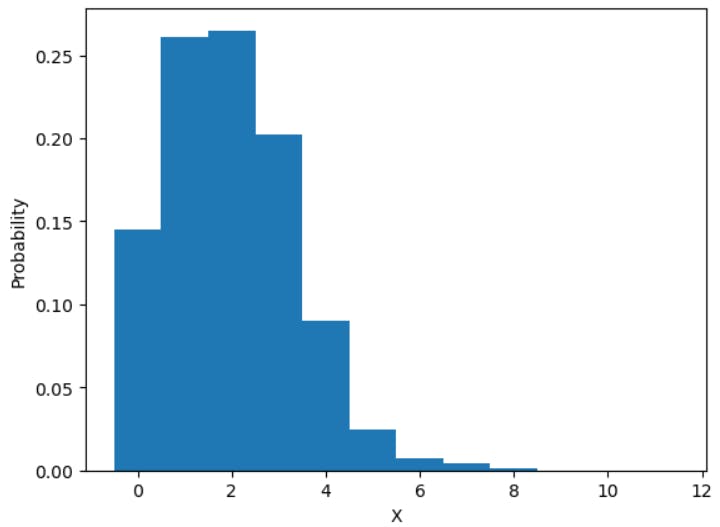
In this example, we used NumPy to simulate 1000 values of X from a Poisson distribution with parameter λ=2. We then plotted a histogram of the simulated values, which shows the probability distribution of X. The histogram closely resembles the theoretical probability mass function of the Poisson distribution, which is a bell-shaped curve with its peak at λ=2.

These are just a few examples of how Python can be used to work with random variables, expectations, and statistical inference. There are many more libraries and functions available in Python that can help with these topics, such as pandas, scipy.stats, and statsmodels.

---

Conclusion:

In this blog post, we introduced the concepts of random variables and expectations, and discussed how they are used in data analysis. We also explained the concepts of variance, covariance, and statistical inference, and provided examples and exercises to help readers better understand these concepts.

Random variables and expectations are important tools in statistics and data analysis, and understanding these concepts can help analysts make better decisions and draw more accurate conclusions from data. Variance and covariance are measures of how much the values of random variables vary from their expected values, and can provide insights into the relationships between different variables.

Statistical inference allows analysts to make conclusions about populations based on sample data, and is a fundamental tool in many areas of data analysis. By mastering these concepts and techniques, analysts can gain a deeper understanding of data and make more informed decisions in a wide range of fields, from finance and economics to healthcare and engineering.